Shallow Neural Networks

Overview

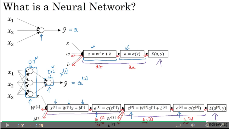
Video #1 says superscript square brackets refers to the layer, as opposed to superscript round brackets which refers to an input sample.

Neural network representation

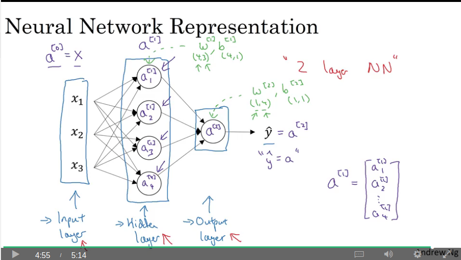
Video #2 mentions input layer (a superscript square bracket zero), hidden layer (a superscript square bracket one, with each neuron having a subscript 1..n), output layer (a superscript square bracket two), and target prediction which is just equal to the last layer. This described a 2-layer network.

Note for a[1] the weights are w[1] of dimension (4,3) and the bias is b[1] with dimension (4,1). The output node has w[2] of (1,4) and b[2] of (1,1).

Computing a neural network’s output

Video #3 says that our new representation of a neural net’s hidden layer contains more than one of the single-node logistic regression node we studied in week 2.

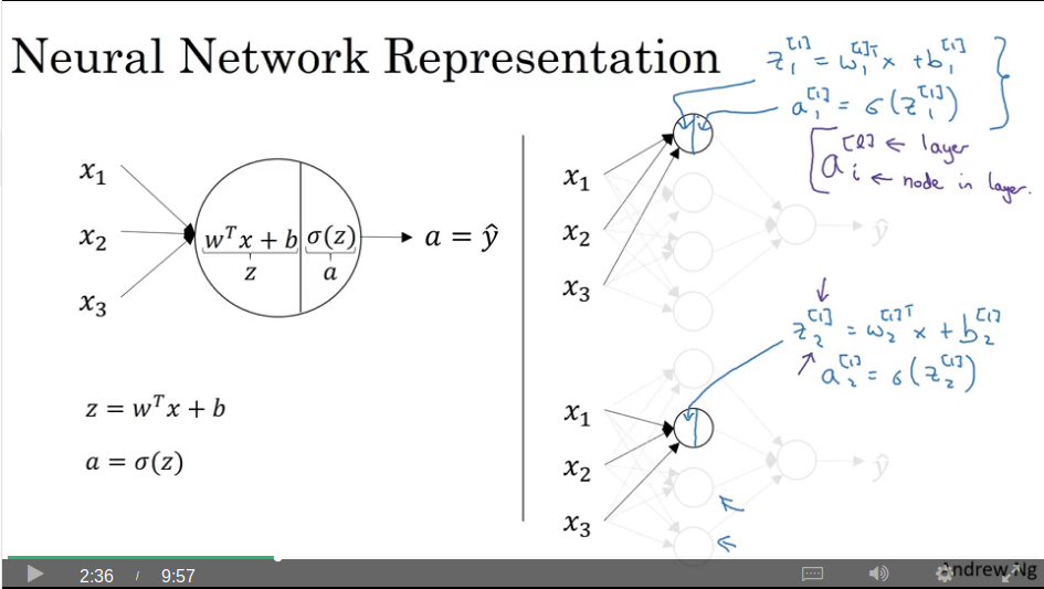
Again, the trick is to not for-loop over the 1+ new nodes, but to vectorise a solution.

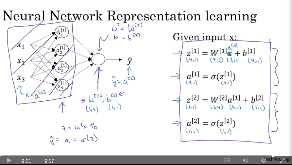
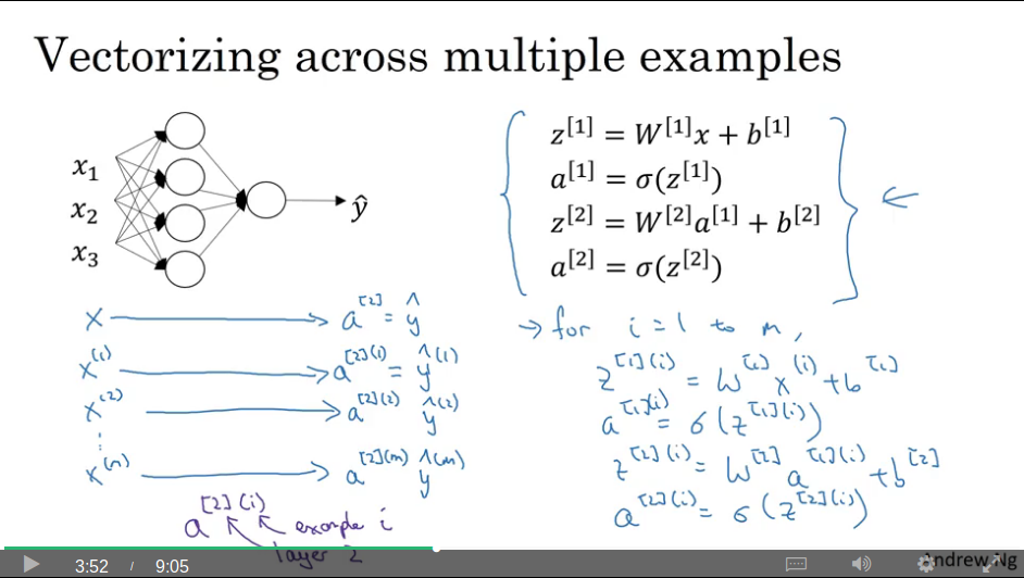
To compute this 2-layer network, you need these 4 formulas:

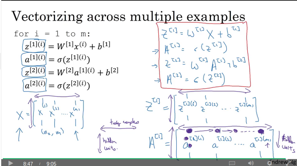
Vectorising across multiple examples

Video #4 is like before, but vectorising across many training examples.

Vectorising the for-loop. A[1]’s first column refers to the first training example, and the first row of the first column refers to the activation in the first hidden node. The next row refers to the activation of the first training example in the second hidden node.

Similarly, A[1]’s second column refers to the second training example, and the first row of the second column refers to the activation of the second training example in the first hidden node, and so forth.

Explanation for vectorised implementation

Video #5 just adds an explanation to the previous concept.

Activation functions

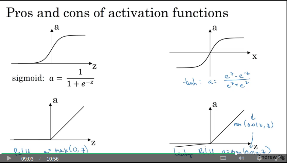
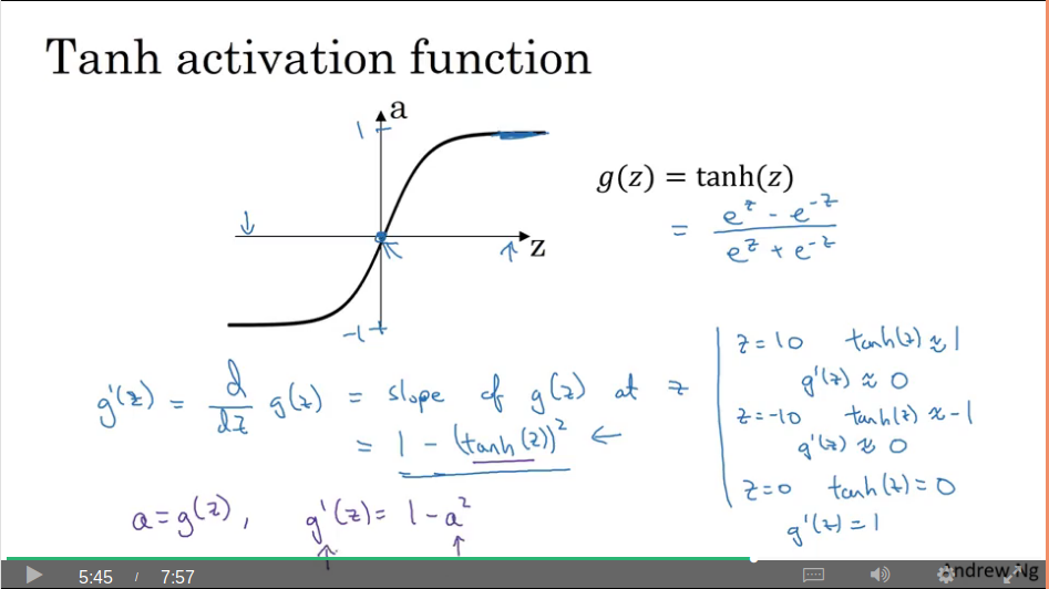
Video #6 notes that thus far in the course we’ve been using sigmoid activation function, but reveals alternatives. The first candidate being tanh or the hyperbolic tangent, which Ng notes is almost always a better choice than sigmoid (because tanh yields a 0 mean, and sigmoid a 0.5 mean, so tanh centers your data, but doesn’t elaborate further)

The exception is to use the sigmoid function on an output layer which does binary classification, where you’d like a prediction between 0 and 1.

The downside to tanh (which is the same for sigmoid) is that the slope is zero when z is very large or very small and this can slow down gradient descent.

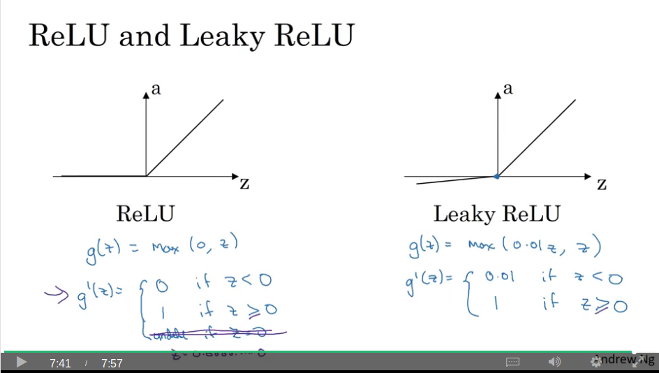
Which brings us to ReLU. The derivative is 0 when z is negative, and for positive z the slope is just very distinct from 0, so your network learns much faster, and this works well in practice.

There’s also “leaky ReLU” which has a slight slope for negative z

Ng ends with a note that we’re spoilt for choice when it comes to which hyperparameters, activations, loss, etc to use, and you have to “try them all” to see which suits your application the best. Time to get a second GPU, then.

Why do you need non-linear activation functions?

Video #7 asks “why need an activation function at all?”

We try and experiment where we just set a to z. yhat then just becomes a linear function of your features x and the model is no more expressive than just standard logistic regression. The hidden layer becomes useless, because a composition of a linear function is itself just a linear function.

However, if your output is a real number (not a classification), e.g. like predicting a house price, then you don’t want a linear activation function.

Derivatives of activation functions

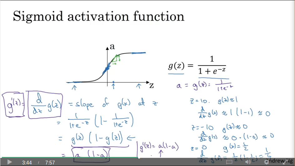
Video #8 reminds us that back-prop uses the slope of the activation functions.

Sigmoid slopes at high and low are 0, and the slope at z=0 is 1/4.

Tanh slope is 0 at high and low, and 1 at z=0.

ReLU has slope 0 for z<0 and 1 for z>=0.

Leaky ReLU has slope 0.01 for z<0 and 1 for z>=0.

Gradient descent for neural networks

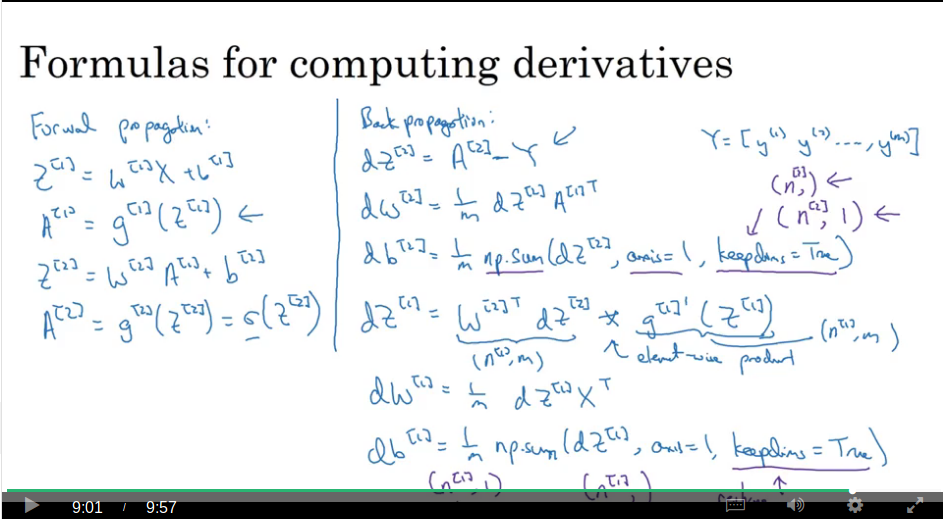
Video #9 is the crib sheet for the formulas for a one hidden layer neural network.

A note on matrix dimensions: For a network with the first layer size nx = n0, the hidden layer size n1, and the output size n2 (or 1), the dimensions will be as follows:

• W1 = (n1, n0)
• b1 = (n1, 1) (aka an n1 dimensional vector, or an n1-by-1 dimensional matrix, or column vector)
• W2 = (n2, n1)
• b2 = (n2, 1)

Backpropagation intuition (optional)

Video #10 explains the cribsheet from the previous video. Worth a watch.

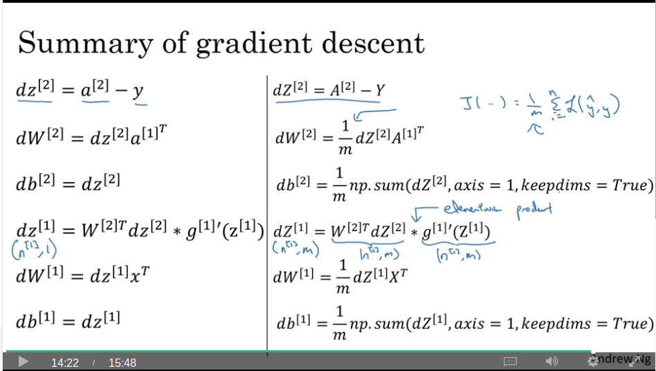
And with that Ng notes that we’ve just seen the most difficult part of neural networks: deriving these functions.

Random initialisation

Video #11 starts of with stating that initialising weights to zero for logistic regression was OK (because it’s single node), but for a neural network it won’t work: you end up with a symmetry problem - all nodes compute the same thing. The bias can be initialised to zero.

# very small random values
W1 = np.random.randn((nx,m)) * 0.01
b1 = np.zero((nx,1))

Why small initial values? Large initial values will be on the outskirts of sigmoid or tanh, and have zero-ish slope, so the network trains very slowly (less of an issue if you don’t use sigmoid or tanh).

0.01 is OK for a shallow network, but next week will discuss why you might want to use smaller values (epsilon?).

What else I’ve learned

The model we built by hand in the previous week’s’ exam can be summarised in these few lines using sklearn:

clf = sklearn.linear_model.LogisticRegressionCV()
clf.fit(X.T, Y.T)
LR_predictions = clf.predict(X.T)

# plot
plot_decision_boundary(lambda x: clf.predict(x), X, Y)
plt.title("Logistic Regression")

Logistic regression doesn’t work on a dataset that isn’t linearly separable. A classification problem IS linearly separable, but we’ll now encounter problems that aren’t.

Neural networks are able to learn even highly non-linear decision boundaries, unlike logistic regression. The techniques learnt during this week can still lead to overfitted models (when using many iterations), but in later weeks we will learn about regularisation, which lets you use very large models (such as n_h = 50) without much overfitting.

References from exam:

http://scs.ryerson.ca/~aharley/neural-networks/ http://cs231n.github.io/neural-networks-case-study/