Introduction to ML Strategy

Why ML Strategy?

Video #1 talks about the motivation: you’ve worked on your cat classifier model, and only achieve 90% accuracy.

You have ideas how to improve:

• collect more data
• collect more diverse training set
• train algo longer with gradient descent
• try Adam instead of gradient descent
• try a bigger/smaller network
• try dropout
• Add L2 regularisation
• change the architecture
  • activation functions
  • hidden units
  • etc

You might choose poorly and waste time.

This course will teach you strategies to point you in the direction of the more promising things to try.

Orthogonalisation

In Video #2 talks about orthogonalisation, which is knowing which change effects which outcome.

An analog is an old-fashion monitor which has distinct knobs for adjusting each of the picture

• width
• height
• trapezoidal shape
• x offset
• y offset
• brightness
• contrast

Now imagine you had only one knob, which - when fiddled adjusts the picture in this way:

0.3 * height + 0.1 * width + 8 * brightness + 0.5 * trapezoidal ... etc

This knob would be impossible to use.

So, Orthogonalisation means that the monitor designers designed the knobs and underlying circuitry so that each knob does only one thing.

The chain of outcomes we’d like to perform well, in order, are:

• fit the training set well on cost function
• fit dev set well on cost function
• fit test set well on cost function
• performs well in real world

Each of these steps would have different “knobs” you can try, e.g.

• “bigger network” or “Adam” for training set
• “regularisation” for dev set
• “bigger dev set” for test set
• “change dev set” or “change cost function” for real world

Ng notes that “early stopping” is less orthogonalised because it changes both how well you fit the training set, because of you stop early, you fit the training set less well. It also improves dev set performance. So, it does two things.

Setting up your goal

Single number evaluation metric

Video #3 shows a single number which you can look at to help you choose a classifier to iterate on.

Example 1

Instead of looking at both Precision and Recall. (Ng mentions don’t worry too much about the definitions for now, hence my own link)

The one number to look at is the F1 score. The hand-wavy way to think of it is the “average of Precision and Recall” says Ng. More accurately, it’s the Harmonic Mean of P and R: 2 / (1/P + 1/R). F1 becomes your single real number evaluation metric.

Example 2

Your app targets four regions, and your classifier gives different error rates for each region. A single real number metric hear could just be the average of those four numbers and then the classifier with the lowest average error is the better one.

A dev set and a single real number evaluation metric will help you make better choices with your classifiers.

Satisficing and Optimising metric

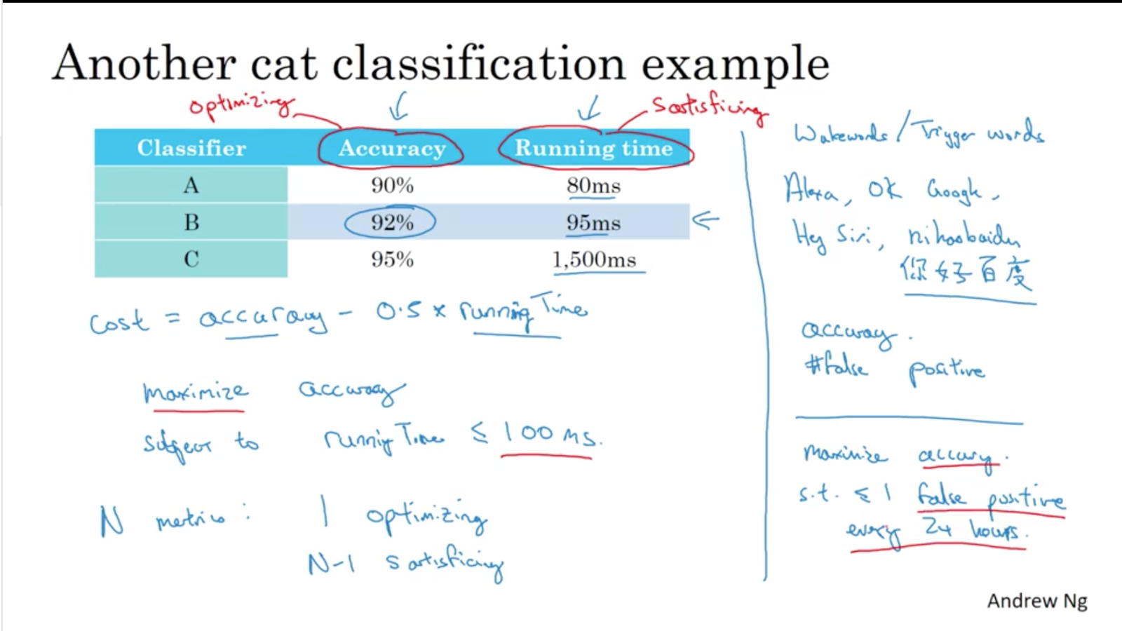
Video #4 shows that you needn’t build a hacky cost function to help you make a decision, e.g. accuracy - 0.5 * running_time, but instead of say something like “I’m happy with any running time below 100ms, after which I’ll choose the most accurate”.

In this case, “running time” is satisficing, and “accuracy” is optimising.

You’ll have one optimising metric, and one or more satisficing metrics.

Train/dev/test set distributions

Video #5 shows the train/dev/test set distributions.

Dev set is aka the “hold-out cross validation set”.

Choose a dev set and test set from the same distribution to reflect the data you expect to see in the future AND consider important to do well on.

E.g. if you’re targetting US and China with your app, don’t make the dev set US, and the test set China, because you’ll end up with moving targets.

Size of dev and test sets

Video #6 shows how old-school heuristics like a 70%/30% split on train/test doesn’t really make sense if you have big data.

Set your test set to be big enough to give high confidence in the overall performance of your system.

The set you’re tuning/iterating on is the dev set, although this was previously called test set. Which brings us to: sometimes you mighn’t need a test set, just a train/dev set, because a large enough dev set means you might not overfit it too badly. Ng says he still prefers a test set in all cases.

When to change dev/test sets and metrics

Video #7 says you might have put your target in the wrong place, so it would be a good idea to move the target, i.e. change the dev/test sets, or redefine the error metric in your code (put a very low weight on porn images so it doesn’t activate a cat prediction).

So far we’ve discussed how to define a metric to evaluate classifiers, but now we’ll talk about how to do well on this metric. Aka we’ve determined where to place the target, but now we’ll focus on how to hit the bull’s eye a bit better. That might be optmising the cost function J that your network is optimising.

Comparing to human-level performance

Why human-level performance?

Video #8 talks about why human-level performance matters as a comparison to machine-level performance.

It talks about Bayes optimal error, the best possible error. E.g. the perfect error might not be zero if an image is just too blurry to classify.

Human tasks are still valuable if the ML is poor, e.g.

• getting labelled data from humans
• manual error analysis
• better analysis of bias/variance (which we’ll talk about later)

Knowing how well humans do can help you reduce bias and variance.

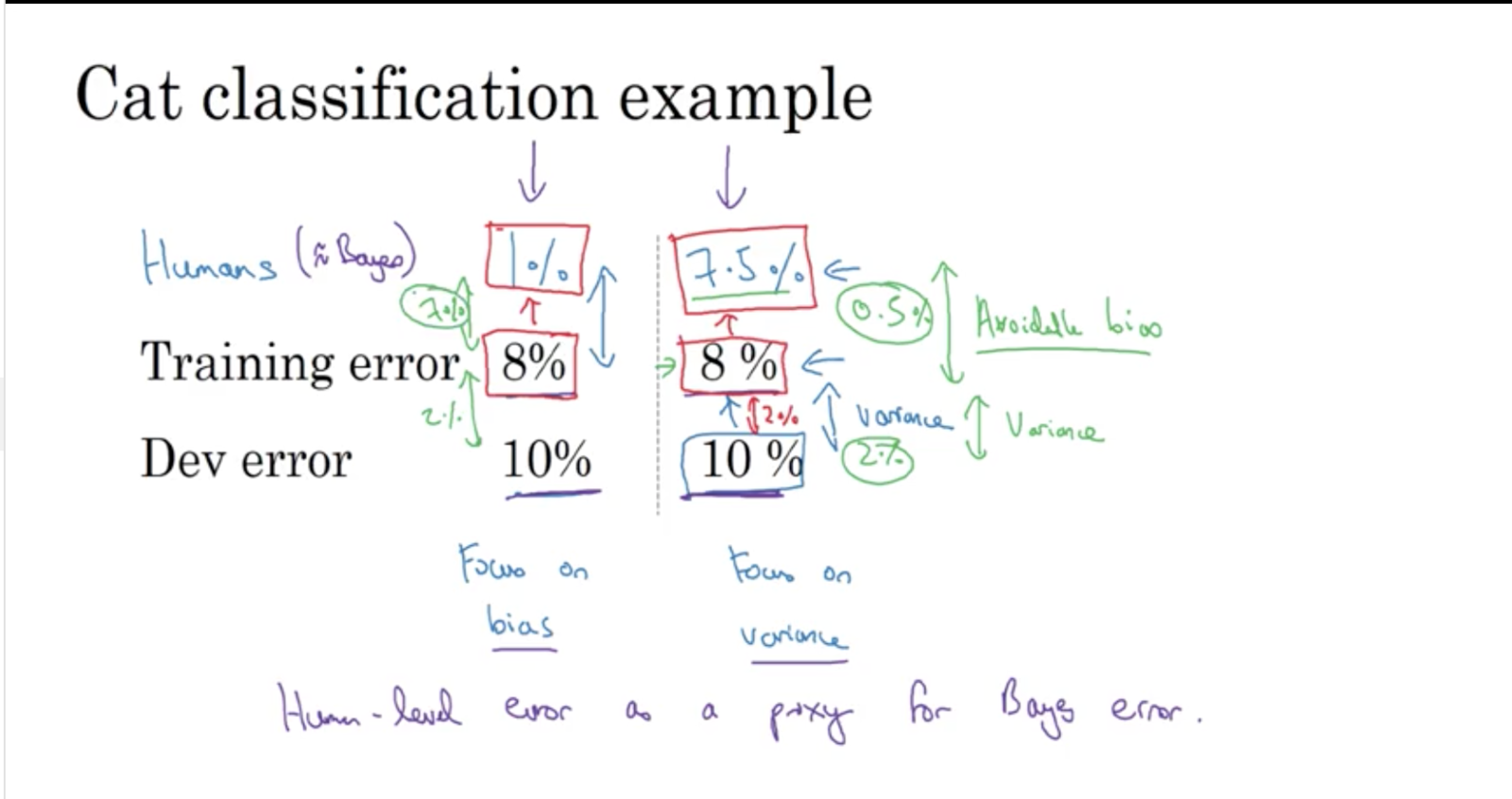
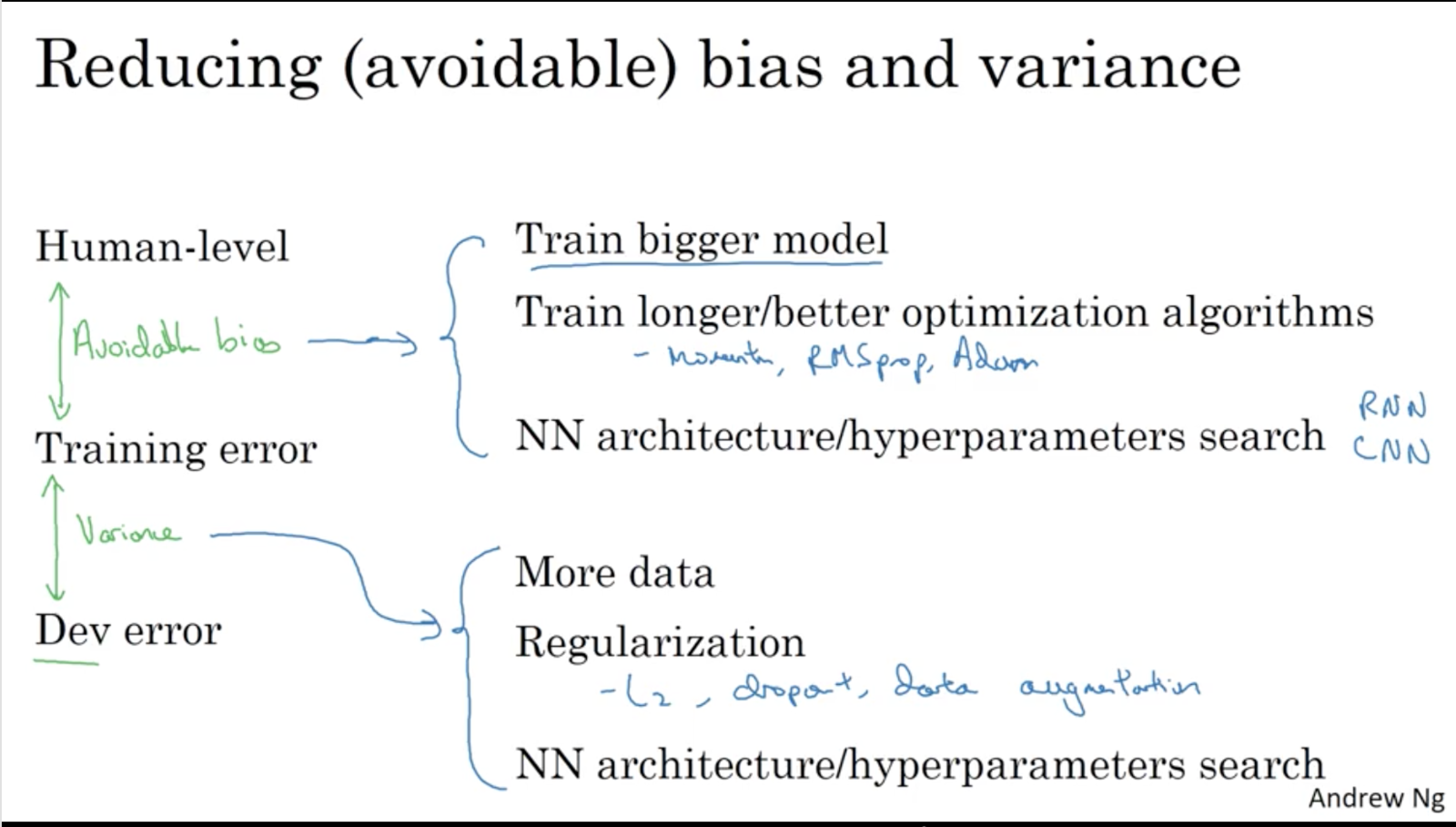
Avoidable bias

Video #9 shows that you can use bias reduction techniques when the human error is much lower than your training error, or variance reduction/avoidance techniques/tactics when the human error is near the training error, but the dev error is still a way off.

Bias reduction techniques could be training a larger network or running the training set for longer.

Variance reduction techniques could be regularisation or increasing the training set.

Human error is a good proxy for Bayes error in image classification, because eyesight our stronger sense.

The difference between human/Bayes error and the training error is called the avoidable bias: keep improving your training performance until you reach Bayes error. (you can’t go further, because Bayes error is the theoretical limit)

The difference between training error and dev error is the variance.

Understanding human-level performance

Video #10 asks how would you define “human level error” if you have a range of humans, e.g. when looking at an X-ray to make a diagnoses, how would Joe Bloggs VS doctor VS experienced doctor VS TEAM of experienced doctors perform and which one of those is your “human level performance”.

Depending on the context, the answer could be to go with the Bayes proxy, i.e. with the lowest error if you want to diagnose correctly. Or the context could be to have a low-level “see a specialist” recommender which could fare as well as a typical doctor.

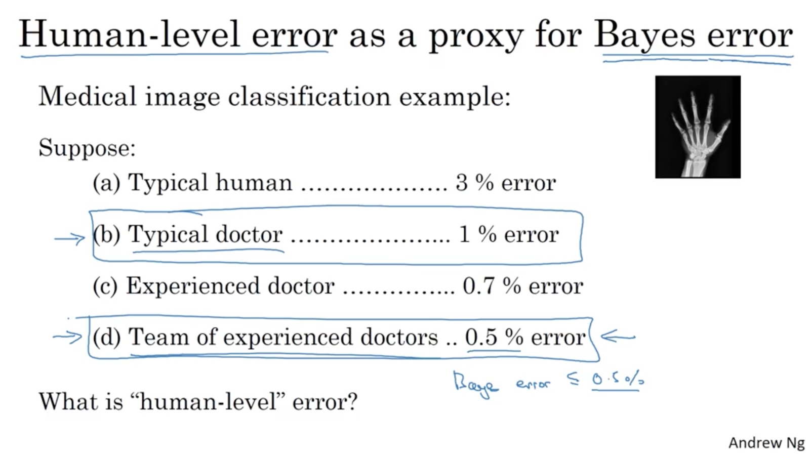
Ng applies this “choice” of humans to the bias/variance decision, e.g. whichever human level you choose, if the training error is far off, focus on avoidable bias.

Surpassing human-level performance

Video #10 mentions that ML surpass humans in structured data problems which aren’t perception tasks. E.g. humans do well with vision and audio, but a machine can clearly fare better at pouring over (lots of) structured data. However, ML is getting better at perception problems too now.

Improving your model performance

Video #11 summaries that we’ve now learned about

• orthogonalisation
• how to set up dev/test sets
• human level performance as a proxy for Bayes error
• how to estimate avoidable bias and variance

This session pulls it together into a set of guidelines:

This week’s Heroes of Deep Learning video features Andrej Karpathy.

And that’s a wrap for week 1.